Five tips to improve your R code
@drsimonj here with five simple tricks I find myself sharing all the time with fellow R users to improve their code!
This post was originally published on DataCamp’s community as one of their top 10 articles in 2017
1. More fun to sequence from 1 #
Next time you use the colon operator to create a sequence from 1 like 1:n, try seq().
# Sequence a vector
x <- runif(10)
seq(x)
#>  [1]  1  2  3  4  5  6  7  8  9 10

# Sequence an integer
seq(nrow(mtcars))
#>  [1]  1  2  3  4  5  6  7  8  9 10 11 12 13 14 15 16 17 18 19 20 21 22 23
#> [24] 24 25 26 27 28 29 30 31 32
The colon operator can produce unexpected results that can create all sorts of problems without you noticing! Take a look at what happens when you want to sequence the length of an empty vector:
# Empty vector
x <- c()

1:length(x)
#> [1] 1 0

seq(x)
#> integer(0)
You’ll also notice that this saves you from using functions like length(). When applied to an object of a certain length, seq() will automatically create a sequence from 1 to the length of the object.
2. vector() what you c() #
Next time you create an empty vector with c(), try to replace it with vector("type", length).
# A numeric vector with 5 elements
vector("numeric", 5)
#> [1] 0 0 0 0 0

# A character vector with 3 elements
vector("character", 3)
#> [1] "" "" ""
Doing this improves memory usage and increases speed! You often know upfront what type of values will go into a vector, and how long the vector will be. Using c() means R has to slowly work both of these things out. So help give it a boost with vector()!
A good example of this value is in a for loop. People often write loops by declaring an empty vector and growing it with c() like this:
x <- c()
for (i in seq(5)) {
  x <- c(x, i)
}
#> x at step 1 : 1
#> x at step 2 : 1, 2
#> x at step 3 : 1, 2, 3
#> x at step 4 : 1, 2, 3, 4
#> x at step 5 : 1, 2, 3, 4, 5
Instead, pre-define the type and length with vector(), and reference positions by index, like this:
n <- 5
x <- vector("integer", n)
for (i in seq(n)) {
  x[i] <- i
}
#> x at step 1 : 1, 0, 0, 0, 0
#> x at step 2 : 1, 2, 0, 0, 0
#> x at step 3 : 1, 2, 3, 0, 0
#> x at step 4 : 1, 2, 3, 4, 0
#> x at step 5 : 1, 2, 3, 4, 5
Here’s a quick speed comparison:
n <- 1e5

x_empty <- c()
system.time(for(i in seq(n)) x_empty <- c(x_empty, i))
#>    user  system elapsed
#>  16.147   2.402  20.158

x_zeros <- vector("integer", n)
system.time(for(i in seq(n)) x_zeros[i] <- i)
#>    user  system elapsed
#>   0.008   0.000   0.009
That should be convincing enough!
3. Ditch the which() #
Next time you use which(), try to ditch it! People often use which() to get indices from some boolean condition, and then select values at those indices. This is not necessary.
Getting vector elements greater than 5:
x <- 3:7

# Using which (not necessary)
x[which(x > 5)]
#> [1] 6 7

# No which
x[x > 5]
#> [1] 6 7
Or counting number of values greater than 5:
# Using which
length(which(x > 5))
#> [1] 2

# Without which
sum(x > 5)
#> [1] 2
Why should you ditch which()? It’s often unnecessary and boolean vectors are all you need.
For example, R lets you select elements flagged as TRUE in a boolean vector:
condition <- x > 5
condition
#> [1] FALSE FALSE FALSE  TRUE  TRUE
x[condition]
#> [1] 6 7
Also, when combined with sum() or mean(), boolean vectors can be used to get the count or proportion of values meeting a condition:
sum(condition)
#> [1] 2
mean(condition)
#> [1] 0.4
which() tells you the indices of TRUE values:
which(condition)
#> [1] 4 5
And while the results are not wrong, it’s just not necessary. For example, I often see people combining which() and length() to test whether any or all values are TRUE. Instead, you just need any() or all():
x <- c(1, 2, 12)

# Using `which()` and `length()` to test if any values are greater than 10
if (length(which(x > 10)) > 0)
  print("At least one value is greater than 10")
#> [1] "At least one value is greater than 10"

# Wrapping a boolean vector with `any()`
if (any(x > 10))
  print("At least one value is greater than 10")
#> [1] "At least one value is greater than 10"

# Using `which()` and `length()` to test if all values are positive
if (length(which(x > 0)) == length(x))
  print("All values are positive")
#> [1] "All values are positive"

# Wrapping a boolean vector with `all()`
if (all(x > 0))
  print("All values are positive")
#> [1] "All values are positive"
Oh, and it saves you a little time…
x <- runif(1e8)

system.time(x[which(x > .5)])
#>    user  system elapsed
#>   1.245   0.486   1.856

system.time(x[x > .5])
#>    user  system elapsed
#>   1.085   0.395   1.541
4. factor that factor! #
Ever removed values from a factor and found you’re stuck with old levels that don’t exist anymore? I see all sorts of creative ways to deal with this. The simplest solution is often just to wrap it in factor() again.
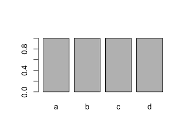
This example creates a factor with four levels ("a", "b", "c" and "d"):
# A factor with four levels
x <- factor(c("a", "b", "c", "d"))
x
#> [1] a b c d
#> Levels: a b c d

plot(x)
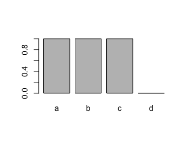
If you drop all cases of one level ("d"), the level is still recorded in the factor:
# Drop all values for one level
x <- x[x != "d"]

# But we still have this level!
x
#> [1] a b c
#> Levels: a b c d

plot(x)
A super simple method for removing it is to use factor() again:
x <- factor(x)
x
#> [1] a b c
#> Levels: a b c

plot(x)
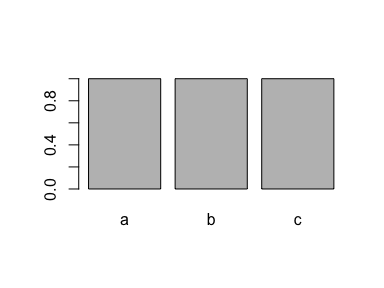
This is typically a good solution to a problem that gets a lot of people mad. So save yourself a headache and factor that factor!
Aside, thanks to Amy Szczepanski who contacted me after the original publication of this article and mentioned
droplevels(). Check it out if this is a problem for you!
5. First you get the $, then you get the power #
Next time you want to extract values from a data.frame column where the rows meet a condition, specify the column with $ before the rows with [.
Examples #
Say you want the horsepower (hp) for cars with 4 cylinders (cyl), using the mtcars data set. You can write either of these:
# rows first, column second - not ideal
mtcars[mtcars$cyl == 4, ]$hp
#>  [1]  93  62  95  66  52  65  97  66  91 113 109

# column first, rows second - much better
mtcars$hp[mtcars$cyl == 4]
#>  [1]  93  62  95  66  52  65  97  66  91 113 109
The tip here is to use the second approach.
But why is that?
First reason: do away with that pesky comma! When you specify rows before the column, you need to remember the comma: mtcars[mtcars$cyl == 4,]$hp. When you specify column first, this means that you’re now referring to a vector, and don’t need the comma!
Second reason: speed! Let’s test it out on a larger data frame:
# Simulate a data frame...
n <- 1e7
d <- data.frame(
  a = seq(n),
  b = runif(n)
)

# rows first, column second - not ideal
system.time(d[d$b > .5, ]$a)
#>    user  system elapsed
#>   0.559   0.152   0.758

# column first, rows second - much better
system.time(d$a[d$b > .5])
#>    user  system elapsed
#>   0.093   0.013   0.107
Worth it, right?
Still, if you want to hone your skills as an R data frame ninja, I suggest learning dplyr. You can get a good overview on the dplyr website or really learn the ropes with online courses like DataCamp’s Data Manipulation in R with dplyr.
Sign off #
Thanks for reading and I hope this was useful for you.
For updates of recent blog posts, follow @drsimonj on Twitter, or email me at drsimonjackson@gmail.com to get in touch.
If you’d like the code that produced this blog, check out the blogR GitHub repository.