corrr 0.2.1 now on CRAN
@drsimonj here to discuss the latest CRAN release of corrr (0.2.1), a package for exploring correlations in a tidy R framework. This post will describe corrr features added since version 0.1.0.
You can install or update to this latest version directly from CRAN by running:
install.packages("corrr")
Let’s load corrr into our workspace and create a correlation data frame of the mtcars data set to work with:
library(corrr)
rdf <- correlate(mtcars)
rdf
#> # A tibble: 11 × 12
#>    rowname        mpg        cyl       disp         hp        drat
#>      <chr>      <dbl>      <dbl>      <dbl>      <dbl>       <dbl>
#> 1      mpg         NA -0.8521620 -0.8475514 -0.7761684  0.68117191
#> 2      cyl -0.8521620         NA  0.9020329  0.8324475 -0.69993811
#> 3     disp -0.8475514  0.9020329         NA  0.7909486 -0.71021393
#> 4       hp -0.7761684  0.8324475  0.7909486         NA -0.44875912
#> 5     drat  0.6811719 -0.6999381 -0.7102139 -0.4487591          NA
#> 6       wt -0.8676594  0.7824958  0.8879799  0.6587479 -0.71244065
#> 7     qsec  0.4186840 -0.5912421 -0.4336979 -0.7082234  0.09120476
#> 8       vs  0.6640389 -0.8108118 -0.7104159 -0.7230967  0.44027846
#> 9       am  0.5998324 -0.5226070 -0.5912270 -0.2432043  0.71271113
#> 10    gear  0.4802848 -0.4926866 -0.5555692 -0.1257043  0.69961013
#> 11    carb -0.5509251  0.5269883  0.3949769  0.7498125 -0.09078980
#> # ... with 6 more variables: wt <dbl>, qsec <dbl>, vs <dbl>, am <dbl>,
#> #   gear <dbl>, carb <dbl>
Plotting functions #
The significant changes involve the rplot() and new network_plot() functions that support the visualisation of your correlations.
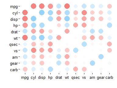
rplot() #
rplot() produces a shape plot of the correlations. More visible dots correspond to stronger correlations, and blue and red respectively to positive and negative. The default plot looks like this:
rplot(rdf)
There are now four arguments that allow you to make adjustments to this plot:
-
legendBoolean indicating whether a legend mapping the colours to the correlations should be displayed. -
shapegeom_point aesthetic. A number corresponding to the shape of each point. See http://sape.inf.usi.ch/quick-reference/ggplot2/shape -
coloursorcolorsVector of colours to use for n-colour gradient. See http://sape.inf.usi.ch/quick-reference/ggplot2/colour -
print_corBoolean indicating whether the correlations should be printed over the shapes.
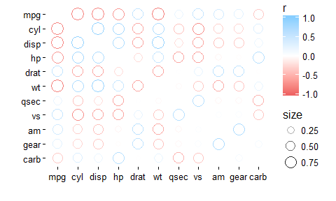
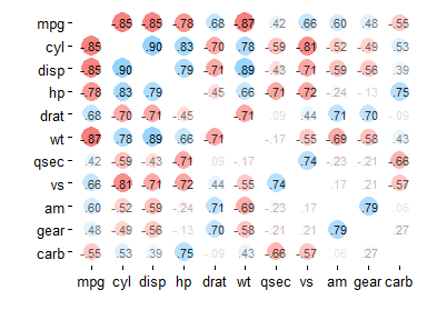
Here are some examples that change these values:
rplot(rdf, legend = TRUE, shape = 1)
rplot(rdf, legend = TRUE, colours = c("firebrick1", "black", "darkcyan"))

rplot(rdf, print_cor = TRUE)
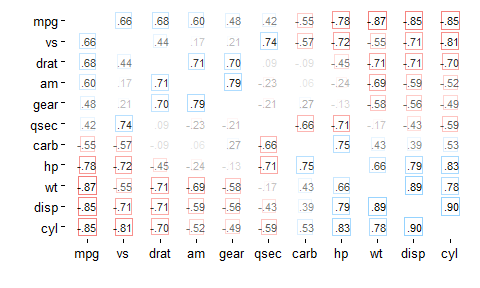
And don’t forget that you can rearrange() your correlations first:
rdf %>% rearrange(absolute = FALSE) %>% rplot(shape = 0, print_cor = TRUE)
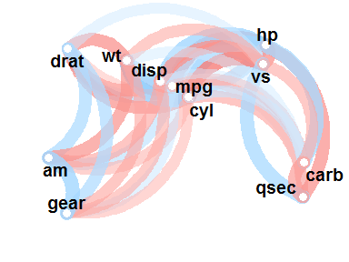
network_plot() #
network_plot() produces a network that lays out and connects variables based on the strength of their correlations:
network_plot(rdf)
For a good intro to network_plot(), see my previous blogR post. Three arguments allow you to adjust this plot:
-
min_corNumber from 0 to 1 indicating the minimum value of correlations (in absolute terms) to plot. -
legendsame asrplot() -
coloursorcolorssame asrplot()
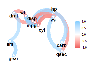
Some examples:
network_plot(rdf, legend = TRUE, colours = c("slategrey", "palegreen"))

network_plot(rdf, legend = TRUE, min_cor = .7)
Other features #
fashion() #
fashion() will now try to work on almost any object (not just correlation data frames). It also provides arguments to adjust the number of decimals, whether to display leading_zeros, and how to print missing values (na_print):
fashion(rdf)
#>    rowname  mpg  cyl disp   hp drat   wt qsec   vs   am gear carb
#> 1      mpg      -.85 -.85 -.78  .68 -.87  .42  .66  .60  .48 -.55
#> 2      cyl -.85       .90  .83 -.70  .78 -.59 -.81 -.52 -.49  .53
#> 3     disp -.85  .90       .79 -.71  .89 -.43 -.71 -.59 -.56  .39
#> 4       hp -.78  .83  .79      -.45  .66 -.71 -.72 -.24 -.13  .75
#> 5     drat  .68 -.70 -.71 -.45      -.71  .09  .44  .71  .70 -.09
#> 6       wt -.87  .78  .89  .66 -.71      -.17 -.55 -.69 -.58  .43
#> 7     qsec  .42 -.59 -.43 -.71  .09 -.17       .74 -.23 -.21 -.66
#> 8       vs  .66 -.81 -.71 -.72  .44 -.55  .74       .17  .21 -.57
#> 9       am  .60 -.52 -.59 -.24  .71 -.69 -.23  .17       .79  .06
#> 10    gear  .48 -.49 -.56 -.13  .70 -.58 -.21  .21  .79       .27
#> 11    carb -.55  .53  .39  .75 -.09  .43 -.66 -.57  .06  .27

fashion(mtcars) %>% head()
#>     mpg  cyl   disp     hp drat   wt  qsec   vs   am gear carb
#> 1 21.00 6.00 160.00 110.00 3.90 2.62 16.46  .00 1.00 4.00 4.00
#> 2 21.00 6.00 160.00 110.00 3.90 2.88 17.02  .00 1.00 4.00 4.00
#> 3 22.80 4.00 108.00  93.00 3.85 2.32 18.61 1.00 1.00 4.00 1.00
#> 4 21.40 6.00 258.00 110.00 3.08 3.21 19.44 1.00  .00 3.00 1.00
#> 5 18.70 8.00 360.00 175.00 3.15 3.44 17.02  .00  .00 3.00 2.00
#> 6 18.10 6.00 225.00 105.00 2.76 3.46 20.22 1.00  .00 3.00 1.00

fashion(c(0.340823, NA, -10.000032), decimals = 3, na_print = "MISSING")
#> [1]    .341 MISSING -10.000

fashion(c(0.340823, NA, -10.000032), leading_zeros = TRUE)
#> [1]   0.34        -10.00
focus() #
A standard evaluation version of focus() is now available, focus_(), to programatically focus on specific correlations:
vars <- c("mpg", "disp")
focus_(rdf, "hp", .dots = vars)
#> # A tibble: 8 × 4
#>   rowname         hp        mpg       disp
#>     <chr>      <dbl>      <dbl>      <dbl>
#> 1     cyl  0.8324475 -0.8521620  0.9020329
#> 2    drat -0.4487591  0.6811719 -0.7102139
#> 3      wt  0.6587479 -0.8676594  0.8879799
#> 4    qsec -0.7082234  0.4186840 -0.4336979
#> 5      vs -0.7230967  0.6640389 -0.7104159
#> 6      am -0.2432043  0.5998324 -0.5912270
#> 7    gear -0.1257043  0.4802848 -0.5555692
#> 8    carb  0.7498125 -0.5509251  0.3949769
Bugs and stuff #
Other than these, there have been fixes to various bugs and minor improvements made to existing functions. Please don’t forget to open an issue on GitHub or email me if you spot an issue or would like a new feature when using corrr.
Acknowledgements #
Many thanks to the community who have already been using corrr and made suggestions along the way. Your help is invaluable for improving corrr!
Sign off #
Thanks for reading and I hope this was useful for you.
For updates of recent blog posts, follow @drsimonj on Twitter, or email me at drsimonjackson@gmail.com to get in touch.
If you’d like the code that produced this blog, check out the blogR GitHub repository.