January 4, 2017

Easy machine learning pipelines with pipelearner: intro and call for contributors

@drsimonj here to introduce pipelearner – a package I’m developing to make it easy to create machine learning pipelines in R – and to spread the word in the hope that some readers may be interested in contributing or testing it.

This post will demonstrate some examples of what pipeleaner can currently do. For example, the Figure below plots the results of a model fitted to 10% to 100% (in 10% increments) of training data in 50 cross-validation pairs. Fitting all of these models takes about four lines of code in pipelearner.

Head to the pipelearner Github page to learn more and contact me if you have a chance to test it yourself or are interested in contributing (my contact details are at the end of this post).

Examples #

Some setup #

library(pipelearner)
library(tidyverse)
library(nycflights13)

# Help functions
r_square <- function(model, data) {
  actual    <- eval(formula(model)[[2]], as.data.frame(data))
  residuals <- predict(model, data) - actual
  1 - (var(residuals, na.rm = TRUE) / var(actual, na.rm = TRUE))
}
add_rsquare <- function(result_tbl) {
  result_tbl %>% 
    mutate(rsquare_train = map2_dbl(fit, train, r_square),
           rsquare_test  = map2_dbl(fit, test,  r_square))
}

# Data set
d <- weather %>%
  select(visib, humid, precip, wind_dir) %>% 
  drop_na() %>%
  sample_n(2000)

# Set theme for plots
theme_set(theme_minimal())

k-fold cross validation #

results <- d %>% 
  pipelearner(lm, visib ~ .) %>% 
  learn_cvpairs(k = 10) %>% 
  learn()

results %>%
  add_rsquare() %>% 
  select(cv_pairs.id, contains("rsquare")) %>% 
  gather(source, rsquare, contains("rsquare")) %>%
  mutate(source = gsub("rsquare_", "", source)) %>% 
  ggplot(aes(cv_pairs.id, rsquare, color = source)) +
    geom_point() +
    labs(x = "Fold",
         y = "R Squared")

Learning curves #

results <- d %>% 
  pipelearner(lm, visib ~ .) %>% 
  learn_curves(seq(.1, 1, .1)) %>% 
  learn()

results %>%
  add_rsquare() %>%
  select(train_p, contains("rsquare")) %>%
  gather(source, rsquare, contains("rsquare")) %>%
  mutate(source = gsub("rsquare_", "", source)) %>% 
  ggplot(aes(train_p, rsquare, color = source)) +
   geom_line() +
   geom_point(size = 2) +
   labs(x = "Proportion of training data used",
       y = "R Squared")

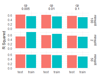
Grid Search #

results <- d %>% 
  pipelearner(rpart::rpart, visib ~ .,
              minsplit = c(2, 50, 100),
              cp = c(.005, .01, .1)) %>% 
  learn()

results %>%
  mutate(minsplit = map_dbl(params, ~ .$minsplit),
         cp       = map_dbl(params, ~ .$cp)) %>% 
  add_rsquare() %>% 
  select(minsplit, cp, contains("rsquare")) %>%
  gather(source, rsquare, contains("rsquare")) %>%
  mutate(source = gsub("rsquare_", "", source),
         minsplit = paste("minsplit", minsplit, sep = "\n"),
         cp       = paste("cp", cp, sep = "\n")) %>% 
  ggplot(aes(source, rsquare, fill = source)) +
   geom_col() +
   facet_grid(minsplit ~ cp) +
   guides(fill = "none") +
   labs(x = NULL, y = "R Squared")

Model comparisons #

results <- d %>% 
  pipelearner() %>% 
  learn_models(
    c(lm, rpart::rpart, randomForest::randomForest),
    visib ~ .) %>% 
  learn()

results %>%
  add_rsquare() %>%
  select(model, contains("rsquare")) %>%
  gather(source, rsquare, contains("rsquare")) %>%
  mutate(source = gsub("rsquare_", "", source)) %>% 
  ggplot(aes(model, rsquare, fill = source)) +
   geom_col(position = "dodge", size = .5) +
   labs(x = NULL, y = "R Squared") +
   coord_flip()

Sign off #

Thanks for reading and I hope this was useful for you.

For updates of recent blog posts, follow @drsimonj on Twitter, or email me at drsimonjackson@gmail.com to get in touch.

If you’d like the code that produced this blog, check out the blogR GitHub repository.

Kudos