k-fold cross validation with modelr and broom
@drsimonj here to discuss how to conduct k-fold cross validation, with an emphasis on evaluating models supported by David Robinson’s broom package. Full credit also goes to David, as this is a slightly more detailed version of his past post, which I read some time ago and felt like unpacking.
Assumed knowledge: K-fold Cross validation #
This post assumes you know what k-fold cross validation is. If you want to brush up, here’s a fantastic tutorial from Stanford University professors Trevor Hastie and Rob Tibshirani.
Creating folds #
Before worrying about models, we can generate K folds using crossv_kfold from the modelr package. Let’s practice with the mtcars data to keep things simple.
library(modelr)
set.seed(1)  # Run to replicate this post
folds <- crossv_kfold(mtcars, k = 5)
folds
#> # A tibble: 5 × 3
#>            train           test   .id
#>           <list>         <list> <chr>
#> 1 <S3: resample> <S3: resample>     1
#> 2 <S3: resample> <S3: resample>     2
#> 3 <S3: resample> <S3: resample>     3
#> 4 <S3: resample> <S3: resample>     4
#> 5 <S3: resample> <S3: resample>     5
This function takes a data frame and randomly partitions it’s rows (1 to 32 for mtcars) into k roughly equal groups. We’ve partitioned the row numbers into k = 5 groups. The results are returned as a tibble (data frame) like the one above.
Each cell in the test column contains a resample object, which is an efficient way of referencing a subset of rows in a data frame (?resample to learn more). Think of each cell as a reference to the rows of the data frame belonging to each partition. For example, the following tells us that the first partition of the data references rows 5, 9, 17, 20, 27, 28, 29, which accounts for roughly 1 / k of the total data set (7 of the 32 rows).
folds$test[[1]]
#> <resample [7 x 11]> 5, 9, 17, 20, 27, 28, 29
Each cell in train also contains a resample object, but referencing the rows in all other partitions. For example, the first train object references all rows except 5, 9, 17, 20, 27, 28, 29:
folds$train[[1]]
#> <resample [25 x 11]> 1, 2, 3, 4, 6, 7, 8, 10, 11, 12, ...
We can now run a model on the data referenced by each train object, and validate the model results on each corresponding partition in test.
Fitting models to training data #
Say we’re interested in predicting Miles Per Gallon (mpg) with all other variables. With the whole data set, we’d do this via:
lm(mpg ~ ., data = mtcars)
Instead, we want to run this model on each set of training data (data referenced in each train cell). We can do this as follows:
library(dplyr)
library(purrr)

folds <- folds %>% mutate(model = map(train, ~ lm(mpg ~ ., data = .)))
folds
#> # A tibble: 5 × 4
#>            train           test   .id    model
#>           <list>         <list> <chr>   <list>
#> 1 <S3: resample> <S3: resample>     1 <S3: lm>
#> 2 <S3: resample> <S3: resample>     2 <S3: lm>
#> 3 <S3: resample> <S3: resample>     3 <S3: lm>
#> 4 <S3: resample> <S3: resample>     4 <S3: lm>
#> 5 <S3: resample> <S3: resample>     5 <S3: lm>
-
folds %>% mutate(model = ...)is adding a newmodelcolumn to the folds tibble. -
map(train, ...)is applying a function to each of the cells intrain -
~ lm(...)is the regression model applied to eachtraincell. -
data = .specifies that the data for the regression model will be the data referenced by eachtrainobject.
The result is a new model column containing fitted regression models based on each of the train data (i.e., the whole data set excluding each partition).
For example, the model fitted to our first set of training data is:
folds$model[[1]] %>% summary()
#>
#> Call:
#> lm(formula = mpg ~ ., data = .)
#>
#> Residuals:
#>     Min      1Q  Median      3Q     Max
#> -3.6540 -0.9116  0.0439  0.9520  4.2811
#>
#> Coefficients:
#>               Estimate Std. Error t value Pr(>|t|)
#> (Intercept) -44.243933  31.884363  -1.388   0.1869
#> cyl           0.844966   1.064141   0.794   0.4404
#> disp          0.016800   0.015984   1.051   0.3110
#> hp            0.004685   0.022741   0.206   0.8398
#> drat          3.950410   1.989177   1.986   0.0670 .
#> wt           -4.487007   2.016341  -2.225   0.0430 *
#> qsec          2.327131   1.243095   1.872   0.0822 .
#> vs           -3.963492   3.217176  -1.232   0.2382
#> am           -0.550804   2.333252  -0.236   0.8168
#> gear          5.476604   2.648708   2.068   0.0577 .
#> carb         -1.595979   1.104272  -1.445   0.1704
#> ---
#> Signif. codes:  0 '***' 0.001 '**' 0.01 '*' 0.05 '.' 0.1 ' ' 1
#>
#> Residual standard error: 2.159 on 14 degrees of freedom
#> Multiple R-squared:  0.9092, Adjusted R-squared:  0.8444
#> F-statistic: 14.02 on 10 and 14 DF,  p-value: 1.205e-05
Predicting the test data #
The next step is to use each model for predicting the outcome variable in the corresponding test data. There are many ways to achieve this. One general approach might be:
folds %>% mutate(predicted = map2(model, test, <FUNCTION_TO_PREDICT_TEST_DATA> ))
map2(model, test, ...) iterates through each model and set of test data in parallel. By referencing these in the function for predicting the test data, this would add a predicted column with the predicted results.
For many common models, an elegant alternative is to use augment from broom. For regression, augment will take a fitted model and a new data frame, and return a data frame of the predicted results, which is what we want! Following above, we can use augment as follows:
library(broom)

folds %>% mutate(predicted = map2(model, test, ~ augment(.x, newdata = .y)))
#> # A tibble: 5 × 5
#>            train           test   .id    model             predicted
#>           <list>         <list> <chr>   <list>                <list>
#> 1 <S3: resample> <S3: resample>     1 <S3: lm> <data.frame [7 × 13]>
#> 2 <S3: resample> <S3: resample>     2 <S3: lm> <data.frame [7 × 13]>
#> 3 <S3: resample> <S3: resample>     3 <S3: lm> <data.frame [6 × 13]>
#> 4 <S3: resample> <S3: resample>     4 <S3: lm> <data.frame [6 × 13]>
#> 5 <S3: resample> <S3: resample>     5 <S3: lm> <data.frame [6 × 13]>
To extract the relevant information from these predicted results, we’ll unnest the data frames thanks to the tidyr package:
library(tidyr)

folds %>%
  mutate(predicted = map2(model, test, ~ augment(.x, newdata = .y))) %>%
  unnest(predicted)
#> # A tibble: 32 × 14
#>      .id   mpg   cyl  disp    hp  drat    wt  qsec    vs    am  gear  carb
#>    <chr> <dbl> <dbl> <dbl> <dbl> <dbl> <dbl> <dbl> <dbl> <dbl> <dbl> <dbl>
#> 1      1  18.7     8 360.0   175  3.15 3.440 17.02     0     0     3     2
#> 2      1  22.8     4 140.8    95  3.92 3.150 22.90     1     0     4     2
#> 3      1  14.7     8 440.0   230  3.23 5.345 17.42     0     0     3     4
#> 4      1  33.9     4  71.1    65  4.22 1.835 19.90     1     1     4     1
#> 5      1  26.0     4 120.3    91  4.43 2.140 16.70     0     1     5     2
#> 6      1  30.4     4  95.1   113  3.77 1.513 16.90     1     1     5     2
#> 7      1  15.8     8 351.0   264  4.22 3.170 14.50     0     1     5     4
#> 8      2  21.0     6 160.0   110  3.90 2.875 17.02     0     1     4     4
#> 9      2  21.4     6 258.0   110  3.08 3.215 19.44     1     0     3     1
#> 10     2  24.4     4 146.7    62  3.69 3.190 20.00     1     0     4     2
#> # ... with 22 more rows, and 2 more variables: .fitted <dbl>,
#> #   .se.fit <dbl>
This was to show you the intermediate steps. In practice we can skip the mutate step:
predicted <- folds %>% unnest(map2(model, test, ~ augment(.x, newdata = .y)))
predicted
#> # A tibble: 32 × 14
#>      .id   mpg   cyl  disp    hp  drat    wt  qsec    vs    am  gear  carb
#>    <chr> <dbl> <dbl> <dbl> <dbl> <dbl> <dbl> <dbl> <dbl> <dbl> <dbl> <dbl>
#> 1      1  18.7     8 360.0   175  3.15 3.440 17.02     0     0     3     2
#> 2      1  22.8     4 140.8    95  3.92 3.150 22.90     1     0     4     2
#> 3      1  14.7     8 440.0   230  3.23 5.345 17.42     0     0     3     4
#> 4      1  33.9     4  71.1    65  4.22 1.835 19.90     1     1     4     1
#> 5      1  26.0     4 120.3    91  4.43 2.140 16.70     0     1     5     2
#> 6      1  30.4     4  95.1   113  3.77 1.513 16.90     1     1     5     2
#> 7      1  15.8     8 351.0   264  4.22 3.170 14.50     0     1     5     4
#> 8      2  21.0     6 160.0   110  3.90 2.875 17.02     0     1     4     4
#> 9      2  21.4     6 258.0   110  3.08 3.215 19.44     1     0     3     1
#> 10     2  24.4     4 146.7    62  3.69 3.190 20.00     1     0     4     2
#> # ... with 22 more rows, and 2 more variables: .fitted <dbl>,
#> #   .se.fit <dbl>
We now have a tibble of the test data for each fold (.id = fold number) and the corresponding .fitted, or predicted values for the outcome variable (mpg) in each case.
Validating the model #
We can compute and examine the residuals:
# Compute the residuals
predicted <- predicted %>%
  mutate(residual = .fitted - mpg)

# Plot actual v residual values
library(ggplot2)
predicted %>%
  ggplot(aes(mpg, residual)) +
    geom_hline(yintercept = 0) +
    geom_point() +
    stat_smooth(method = "loess") +
    theme_minimal()

It looks like our models could be overestimating mpg around 20-30 and underestimating higher mpg. But there are clearly fewer data points, making prediction difficult.
We can also use these values to calculate the overall proportion of variance accounted for by each model:
rs <- predicted %>%
  group_by(.id) %>%
  summarise(
    sst = sum((mpg - mean(mpg)) ^ 2), # Sum of Squares Total
    sse = sum(residual ^ 2),          # Sum of Squares Residual/Error
    r.squared = 1 - sse / sst         # Proportion of variance accounted for
    )
rs
#> # A tibble: 5 × 4
#>     .id      sst       sse r.squared
#>   <chr>    <dbl>     <dbl>     <dbl>
#> 1     1 321.5886 249.51370 0.2241214
#> 2     2 127.4371  31.86994 0.7499164
#> 3     3 202.6600  42.19842 0.7917773
#> 4     4 108.4733  50.79684 0.5317113
#> 5     5 277.3283  59.55946 0.7852385

# Overall
mean(rs$r.squared)
#> [1] 0.616553
So, across the folds, the regression models have accounted for an average of 61.66% of the variance of mpg in new, test data.
Plotting these results:
rs %>%
  ggplot(aes(r.squared, fill  = .id)) +
    geom_histogram() +
    geom_vline(aes(xintercept = mean(r.squared)))  # Overall mean
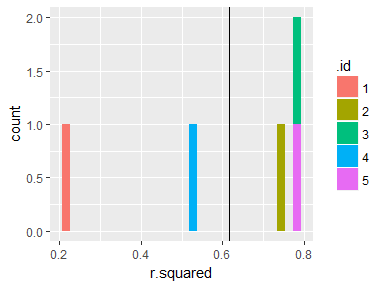
Although the model performed well on average, it performed pretty poorly when fold 1 was used as test data.
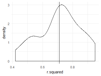
All at once #
With this new knowledge, we can do something similar to the k = 20 case shown in David’s post. See that you can understand what’s going on here:
set.seed(1)
# Select four variables from the mpg data set in ggplot2
ggplot2::mpg %>% select(year, cyl, drv, hwy) %>%
  # Create 20 folds (5% of the data in each partition)
  crossv_kfold(k = 20) %>%
  # Fit a model to training data
  mutate(model = map(train, ~ lm(hwy ~ ., data = .))) %>%
  # Unnest predicted values on test data
  unnest(map2(model, test, ~ augment(.x, newdata = .y))) %>%
  # Compute R-squared values for each partition
  group_by(.id) %>%
  summarise(
    sst = sum((hwy - mean(hwy)) ^ 2),
    sse = sum((hwy - .fitted) ^ 2),
    r.squared = 1 - sse / sst
  ) %>%
  # Plot
  ggplot(aes(r.squared)) +
    geom_density() +
    geom_vline(aes(xintercept = mean(r.squared))) +
    theme_minimal()
Sign off #
Thanks for reading and I hope this was useful for you.
For updates of recent blog posts, follow @drsimonj on Twitter, or email me at drsimonjackson@gmail.com to get in touch.
If you’d like the code that produced this blog, check out the blogR GitHub repository.