Plotting my trips with ubeR
@drsimonj here to explain how I used ubeR, an R package for the Uber API, to create this map of my trips over the last couple of years:
Getting ubeR #
The ubeR package, which I first heard about here, is currently available on GitHub. In R, install and load it as follows:
# install.packages("devtools")  # Run to install the devtools package if needed
devtools::install_github("DataWookie/ubeR")  # Install ubeR
library(ubeR)
For this post I also use many of the tidyverse packages, so install and load this too to follow along:
library(tidyverse)
Setting up an app #
To use ubeR and the uber API, you’ll need an uber account and to register a new app. In a web browser, log into your uber account and head to this page. Fill in the details. Here’s an example:

Once created, under the Authorization tab, set the Redirect URL to http://localhost:1410/

Further down, under General Scopes, enable “profile” and “history”:

Back under the settings tab, under Authentication, take note of the “Client ID” and “Client Secret”:

In your R session, save these values as two variables:
UBER_CLIENTID <- "<< Your App's Client ID >>"
UBER_CLIENTSECRET <- "<< Your App's Client Secret >>"
Using ubeR #
Back in R, run the following:
uber_oauth(UBER_CLIENTID, UBER_CLIENTSECRET)
A web page will open asking you to log in to your uber account and permit the app to access your data. It will then say:
Authentication complete. Please close this page and return to R.
We can now access our uber data via the R functions that access the uber API. For example uber_me() returns a vector of information contained in your profile.
me <- uber_me()
names(me)
#> [1] "email"           "first_name"      "last_name"       "mobile_verified"
#> [5] "picture"         "promo_code"      "rider_id"        "uuid"

cat("My uber profile name is", me$first_name, me$last_name)
#> My uber profile name is Simon Jackson
Accessing trip history #
The function uber_history will return a data frame of portions of your trip history. As far as I can tell, you can extract up to 50 trips at a time. You can use uber_history to return one chunk of up to 50 trips. Alternatively, the following will read all of your trips into a data frame:
trips <- data.frame()
more_trips <- TRUE
off_set <- 0
while(more_trips) {
  new_trips <- uber_history(50, 50 * off_set)
  if (is.null(new_trips)) {
    more_trips <- FALSE
  } else {
    trips <- rbind(trips, new_trips)
    off_set <- off_set + 1
  }
}
trips %>%
  mutate(longitude = "xx", latitude = "yy") %>%  # Just to hide values
  head
#>      status  distance                           product_id
#> 1 completed  8.557486 2d1d002b-d4d0-4411-98e1-673b244878b2
#> 2 completed  4.037542 2d1d002b-d4d0-4411-98e1-673b244878b2
#> 3 completed  6.808492 2d1d002b-d4d0-4411-98e1-673b244878b2
#> 4 completed  2.939439 2d1d002b-d4d0-4411-98e1-673b244878b2
#> 5 completed  2.296352 2d1d002b-d4d0-4411-98e1-673b244878b2
#> 6 completed 13.008353 893b94af-ca9d-4f0f-9201-6d426cedaa5c
#>            start_time            end_time
#> 1 2016-11-25 19:03:43 2016-11-25 19:29:30
#> 2 2016-11-25 15:56:30 2016-11-25 16:22:04
#> 3 2016-11-25 08:18:57 2016-11-25 08:50:18
#> 4 2016-11-20 20:41:20 2016-11-20 20:54:37
#> 5 2016-11-20 18:47:21 2016-11-20 18:57:08
#> 6 2016-11-19 16:04:40 2016-11-19 16:44:33
#>                             request_id        request_time latitude
#> 1 53ef8fc0-c9e9-4879-bd72-1a5ccbca5439 2016-11-25 19:00:46       yy
#> 2 253bc0b3-2df0-41b0-a1e0-f857b6d8feb4 2016-11-25 15:52:56       yy
#> 3 e92525fe-b5c3-42a1-ae16-b7d9047618d6 2016-11-25 08:14:22       yy
#> 4 5a57698c-1d1c-460f-91e5-2425efb7adb9 2016-11-20 20:39:43       yy
#> 5 0c8edfea-55cc-41fc-8966-be479ac7836a 2016-11-20 18:41:18       yy
#> 6 703d4808-5a35-447a-862c-23f683e336ef 2016-11-19 15:57:54       yy
#>   display_name longitude
#> 1       Sydney        xx
#> 2       Sydney        xx
#> 3       Sydney        xx
#> 4       Sydney        xx
#> 5       Sydney        xx
#> 6    Melbourne        xx

# How many trips have I taken?
nrow(trips)
#> [1] 132

# Time and place of my first trip
trips %>%
  filter(start_time == min(start_time)) %>%
  select(start_time, display_name)
#>            start_time display_name
#> 1 2014-12-18 05:34:30       Sydney
Getting the data into shape #
For the map shown at the beginning, I created two data frames from my trip history:
- A data frame of how many trips I’d taken in each city, as well as an estimate of the city longitude and latitude.
- A data frame of transitions from one city to another, along with their longitudes and latitudes.
Trips per city #
Calculating the trips per city is pretty straight forward. Given that we’re using a world map, we can average the longitude and latitude for each city to get a good-enough position.
city_trips <- trips %>%
  group_by(display_name) %>%
  summarise(
    n = n(),
    long = mean(longitude),
    lat = mean(latitude)
  )
city_trips
#> # A tibble: 9 × 4
#>   display_name     n     long      lat
#>          <chr> <int>    <dbl>    <dbl>
#> 1     Adelaide     1 138.6019 -34.9229
#> 2      Chicago     4 -87.6298  41.8781
#> 3       Dallas     6 -96.7699  32.8030
#> 4    Melbourne    15 144.9700 -37.8100
#> 5        Miami    11 -80.2264  25.7890
#> 6   New Jersey     7 -74.0391  40.7710
#> 7  New Orleans     8 -90.1029  29.9555
#> 8 Philadelphia     3 -75.1638  39.9523
#> 9       Sydney    77 151.2076 -33.8705
City-to-city travel paths #
The data comes with dates and is ordered from most recent to oldest. We can use this to approximately work out which cities I’ve gone from and to.
To get my travel paths, we find all occasions where the city for one trip doesn’t match the city for the next trip. We then use the longitude and latitude from city_trips to create x, y, xend, and yend for the paths that we’ll draw on the map.
travel_paths <- trips %>%
  # Find the from-to travel paths
  select(display_name) %>%
  rename(from = display_name) %>%
  mutate(to = lag(from)) %>%
  filter(from != to) %>%
  filter(!duplicated(.)) %>%
  # Add coords for from city
  left_join(select(city_trips, -n), by = c("from" = "display_name")) %>%
  rename(x = long, y = lat) %>%
  # Add coords for to city
  left_join(select(city_trips, -n), by = c("to" = "display_name")) %>%
  rename(xend = long, yend = lat)

travel_paths
#>            from           to        x        y     xend     yend
#> 1     Melbourne       Sydney 144.9700 -37.8100 151.2076 -33.8705
#> 2        Sydney    Melbourne 151.2076 -33.8705 144.9700 -37.8100
#> 3      Adelaide       Sydney 138.6019 -34.9229 151.2076 -33.8705
#> 4        Sydney     Adelaide 151.2076 -33.8705 138.6019 -34.9229
#> 5       Chicago       Sydney -87.6298  41.8781 151.2076 -33.8705
#> 6   New Orleans      Chicago -90.1029  29.9555 -87.6298  41.8781
#> 7         Miami  New Orleans -80.2264  25.7890 -90.1029  29.9555
#> 8        Dallas        Miami -96.7699  32.8030 -80.2264  25.7890
#> 9        Sydney       Dallas 151.2076 -33.8705 -96.7699  32.8030
#> 10   New Jersey       Sydney -74.0391  40.7710 151.2076 -33.8705
#> 11 Philadelphia   New Jersey -75.1638  39.9523 -74.0391  40.7710
#> 12   New Jersey Philadelphia -74.0391  40.7710 -75.1638  39.9523
#> 13       Sydney   New Jersey 151.2076 -33.8705 -74.0391  40.7710
Plotting on the map (first attempt) #
The following overlays the data onto the default map with the size of the points for each city determined by the number of trips I’ve taken there:
library(ggrepel)

world_map <-  map_data(map = "world")

ggplot(city_trips, aes(long, lat)) +
  # Plot map
  geom_map(data = world_map, map = world_map,
           aes(map_id = region, x = long, y = lat),
           fill = "gray93", color = "gray85") +
  # Plot travel paths
  geom_curve(data = travel_paths, color = "dodgerblue1",
             aes(x = x, y = y, xend = xend, yend = yend),
             arrow = arrow(angle = 20, type = "closed", length = unit(.18, "inches"))) +
  # Plot city names
  geom_text_repel(aes(label = display_name), force = 20, color = "black", size = 2.5) +
  # Plot city points
  geom_point(aes(size = n), color = "dodgerblue3") +
  # Adjustments
  guides(size = "none", color = "none", alpha = "none") +
  coord_equal() +
  theme_void()
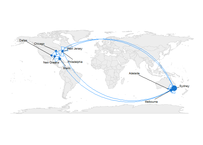
This is pretty good! However, I live in Australia, and I’ve only used uber internationally in the US.
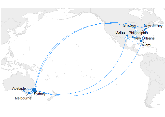
Plotting on a localized map #
To display my trip information a little more clearly, the following creates a local version of the map:
long_min <- 120
long_max <- 300

local_map <- world_map %>%
  mutate(long = long + 360,
         group = group + max(group) + 1) %>%
  rbind(world_map)

local_trips <- city_trips %>%
  mutate(long = long + 360) %>%
  rbind(city_trips)

local_paths <- travel_paths %>%
  mutate(x = x + 360,
         xend = xend + 360) %>%
  rbind(travel_paths) %>%
  group_by(from, to) %>%
  summarise(
    x = x[between(x, long_min, long_max)],
    xend = xend[between(xend, long_min, long_max)],
    y = y[1],
    yend = yend[1]
  )

ggplot(local_trips, aes(long, lat)) +
  geom_map(data = local_map, map = local_map,
           aes(map_id = region, x = long, y = lat),
           fill = "gray93", color = "gray85") +
  geom_curve(data = local_paths, color = "dodgerblue1",
             aes(x = x, y = y, xend = xend, yend = yend),
             arrow = arrow(angle = 20, type = "closed", length = unit(.18, "inches"))) +
  ggrepel::geom_text_repel(aes(label = display_name), force = 10, color = "black") +
  geom_point(aes(size = n), color = "dodgerblue3") +
  guides(size = "none", color = "none", alpha = "none") +
  coord_equal() +
  scale_x_continuous(limits = c(long_min, long_max)) +
  scale_y_continuous(limits = c(-50, 60)) +
  theme_void()

A brief explanation of my trips:
- I live in Sydney, Australia, so most of my uber trips are there.
- I frequently travel to Melbourne to visit family.
- I often work in Adelaide, but usually hire a car, so don’t use uber much while I’m there.
- I did a summer internship at ETS in Princeton, so that included my trip through New Jersey and Philadelphia.
- After finishing my Ph.D. I took a trip around the US, which involved Dallas, Miami, New Orleans, and – my inner nerd couldn’t resist – a conference in Chicago before coming home.
It’s not a complete travel history, but pretty cool to see just through my use of uber!
Sign off #
Thanks for reading and I hope this was useful for you.
For updates of recent blog posts, follow @drsimonj on Twitter, or email me at drsimonjackson@gmail.com to get in touch.
If you’d like the code that produced this blog, check out the blogR GitHub repository.