How and when: ridge regression with glmnet
@drsimonj here to show you how to conduct ridge regression (linear regression with L2 regularization) in R using the glmnet package, and use simulations to demonstrate its relative advantages over ordinary least squares regression.
Ridge regression #
Ridge regression uses L2 regularisation to weight/penalise residuals when the parameters of a regression model are being learned. In the context of linear regression, it can be compared to Ordinary Least Square (OLS). OLS defines the function by which parameter estimates (intercepts and slopes) are calculated. It involves minimising the sum of squared residuals. L2 regularisation is a small addition to the OLS function that weights residuals in a particular way to make the parameters more stable. The outcome is typically a model that fits the training data less well than OLS but generalises better because it is less sensitive to extreme variance in the data such as outliers.
Packages #
We’ll make use of the following packages in this post:
library(tidyverse)
library(broom)
library(glmnet)
Ridge regression with glmnet #
The glmnet package provides the functionality for ridge regression via glmnet(). Important things to know:
- Rather than accepting a formula and data frame, it requires a vector input and matrix of predictors.
- You must specify
alpha = 0for ridge regression. - Ridge regression involves tuning a hyperparameter, lambda.
glmnet()will generate default values for you. Alternatively, it is common practice to define your own with thelambdaargument (which we’ll do).
Here’s an example using the mtcars data set:
y <- mtcars$hp
x <- mtcars %>% select(mpg, wt, drat) %>% data.matrix()
lambdas <- 10^seq(3, -2, by = -.1)

fit <- glmnet(x, y, alpha = 0, lambda = lambdas)
summary(fit)
#>           Length Class     Mode
#> a0         51    -none-    numeric
#> beta      153    dgCMatrix S4
#> df         51    -none-    numeric
#> dim         2    -none-    numeric
#> lambda     51    -none-    numeric
#> dev.ratio  51    -none-    numeric
#> nulldev     1    -none-    numeric
#> npasses     1    -none-    numeric
#> jerr        1    -none-    numeric
#> offset      1    -none-    logical
#> call        5    -none-    call
#> nobs        1    -none-    numeric
Because, unlike OLS regression done with lm(), ridge regression involves tuning a hyperparameter, lambda, glmnet() runs the model many times for different values of lambda. We can automatically find a value for lambda that is optimal by using cv.glmnet() as follows:
cv_fit <- cv.glmnet(x, y, alpha = 0, lambda = lambdas)
cv.glmnet() uses cross-validation to work out how well each model generalises, which we can visualise as:
plot(cv_fit)
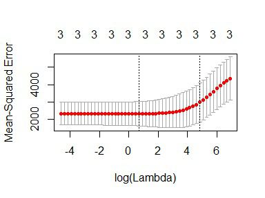
The lowest point in the curve indicates the optimal lambda: the log value of lambda that best minimised the error in cross-validation. We can extract this values as:
opt_lambda <- cv_fit$lambda.min
opt_lambda
#> [1] 3.162278
And we can extract all of the fitted models (like the object returned by glmnet()) via:
fit <- cv_fit$glmnet.fit
summary(fit)
#>           Length Class     Mode
#> a0         51    -none-    numeric
#> beta      153    dgCMatrix S4
#> df         51    -none-    numeric
#> dim         2    -none-    numeric
#> lambda     51    -none-    numeric
#> dev.ratio  51    -none-    numeric
#> nulldev     1    -none-    numeric
#> npasses     1    -none-    numeric
#> jerr        1    -none-    numeric
#> offset      1    -none-    logical
#> call        5    -none-    call
#> nobs        1    -none-    numeric
These are the two things we need to predict new data. For example, predicting values and computing an R2 value for the data we trained on:
y_predicted <- predict(fit, s = opt_lambda, newx = x)

# Sum of Squares Total and Error
sst <- sum((y - mean(y))^2)
sse <- sum((y_predicted - y)^2)

# R squared
rsq <- 1 - sse / sst
rsq
#> [1] 0.9318896
The optimal model has accounted for 93% of the variance in the training data.
Ridge v OLS simulations #
By producing more stable parameters than OLS, ridge regression should be less prone to overfitting training data. Ridge regression might, therefore, predict training data less well than OLS, but better generalise to new data. This will particularly be the case when extreme variance in the training data is high, which tends to happen when the sample size is low and/or the number of features is high relative to the number of observations.
Below is a simulation experiment I created to compare the prediction accuracy of ridge regression and OLS on training and test data.
I first set up the functions to run the simulation:
# Compute R^2 from true and predicted values
rsquare <- function(true, predicted) {
  sse <- sum((predicted - true)^2)
  sst <- sum((true - mean(true))^2)
  rsq <- 1 - sse / sst

  # For this post, impose floor...
  if (rsq < 0) rsq <- 0

  return (rsq)
}

# Train ridge and OLS regression models on simulated data set with `n_train`
# observations and a number of features as a proportion to `n_train`,
# `p_features`. Return R squared for both models on:
#   - y values of the training set
#   - y values of a simualted test data set of `n_test` observations
#   - The beta coefficients used to simulate the data
ols_vs_ridge <- function(n_train, p_features, n_test = 200) {
  ## Simulate datasets
  n_features <- floor(n_train * p_features)
  betas <- rnorm(n_features)

  x <- matrix(rnorm(n_train * n_features), nrow = n_train)
  y <- x %*% betas + rnorm(n_train)
  train <- data.frame(y = y, x)

  x <- matrix(rnorm(n_test * n_features), nrow = n_test)
  y <- x %*% betas + rnorm(n_test)
  test <- data.frame(y = y, x)

  ## OLS
  lm_fit <- lm(y ~ ., train)

  # Match to beta coefficients
  lm_betas <- tidy(lm_fit) %>%
    filter(term != "(Intercept)") %>%
    {.$estimate}
  lm_betas_rsq <- rsquare(betas, lm_betas)

  # Fit to training data
  lm_train_rsq <- glance(lm_fit)$r.squared

  # Fit to test data
  lm_test_yhat <- predict(lm_fit, newdata = test)
  lm_test_rsq  <- rsquare(test$y, lm_test_yhat)

  ## Ridge regression
  lambda_vals <- 10^seq(3, -2, by = -.1)  # Lambda values to search
  cv_glm_fit  <- cv.glmnet(as.matrix(train[,-1]), train$y, alpha = 0, lambda = lambda_vals, nfolds = 5)
  opt_lambda  <- cv_glm_fit$lambda.min  # Optimal Lambda
  glm_fit     <- cv_glm_fit$glmnet.fit

  # Match to beta coefficients
  glm_betas <- tidy(glm_fit) %>%
    filter(term != "(Intercept)", lambda == opt_lambda) %>%
    {.$estimate}
  glm_betas_rsq <- rsquare(betas, glm_betas)

  # Fit to training data
  glm_train_yhat <- predict(glm_fit, s = opt_lambda, newx = as.matrix(train[,-1]))
  glm_train_rsq  <- rsquare(train$y, glm_train_yhat)

  # Fit to test data
  glm_test_yhat <- predict(glm_fit, s = opt_lambda, newx = as.matrix(test[,-1]))
  glm_test_rsq  <- rsquare(test$y, glm_test_yhat)

  data.frame(
    model = c("OLS", "Ridge"),
    betas_rsq  = c(lm_betas_rsq, glm_betas_rsq),
    train_rsq = c(lm_train_rsq, glm_train_rsq),
    test_rsq = c(lm_test_rsq, glm_test_rsq)
  )

}

# Function to run `ols_vs_ridge()` `n_replications` times
repeated_comparisons <- function(..., n_replications = 5) {
  map(seq(n_replications), ~ ols_vs_ridge(...)) %>%
    map2(seq(.), ~ mutate(.x, replicate = .y)) %>%
    reduce(rbind)
}
Now run the simulations for varying numbers of training data and relative proportions of features (takes some time):
d <- purrr::cross_d(list(
  n_train = seq(20, 200, 20),
  p_features = seq(.55, .95, .05)
))

d <- d %>%
  mutate(results = map2(n_train, p_features, repeated_comparisons))
Visualise the results…
For varying numbers of training data (averaging over number of features), how well do both models predict the training and test data?
d %>%
  unnest() %>%
  group_by(model, n_train) %>%
  summarise(
    train_rsq = mean(train_rsq),
    test_rsq = mean(test_rsq)) %>%
  gather(data, rsq, contains("rsq")) %>%
  mutate(data = gsub("_rsq", "", data)) %>%
  ggplot(aes(n_train, rsq, color = model)) +
    geom_line() +
    geom_point(size = 4, alpha = .3) +
    facet_wrap(~ data) +
    theme_minimal() +
    labs(x = "Number of training observations",
         y = "R squared")
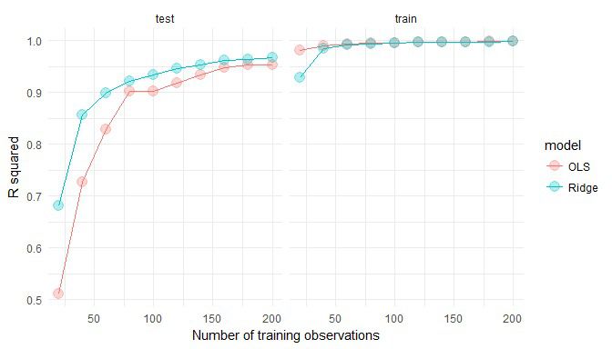
As hypothesised, OLS fits the training data better but Ridge regression better generalises to new test data. Further, these effects are more pronounced when the number of training observations is low.
For varying relative proportions of features (averaging over numbers of training data) how well do both models predict the training and test data?
d %>%
  unnest() %>%
  group_by(model, p_features) %>%
  summarise(
    train_rsq = mean(train_rsq),
    test_rsq = mean(test_rsq)) %>%
  gather(data, rsq, contains("rsq")) %>%
  mutate(data = gsub("_rsq", "", data)) %>%
  ggplot(aes(p_features, rsq, color = model)) +
    geom_line() +
    geom_point(size = 4, alpha = .3) +
    facet_wrap(~ data) +
    theme_minimal() +
    labs(x = "Number of features as proportion\nof number of observation",
         y = "R squared")

Again, OLS has performed slightly better on training data, but Ridge better on test data. The effects are more pronounced when the number of features is relatively high compared to the number of training observations.
The following plot helps to visualise the relative advantage (or disadvantage) of Ridge to OLS over the number of observations and features:
d %>%
  unnest() %>%
  group_by(model, n_train, p_features) %>%
  summarise(train_rsq = mean(train_rsq),
            test_rsq  = mean(test_rsq)) %>%
  group_by(n_train, p_features) %>%
  summarise(RidgeAdvTrain = train_rsq[model == "Ridge"] - train_rsq[model == "OLS"],
            RidgeAdvTest  = test_rsq[model == "Ridge"] - test_rsq[model == "OLS"]) %>%
  gather(data, RidgeAdvantage, contains("RidgeAdv")) %>%
  mutate(data = gsub("RidgeAdv", "", data)) %>%
  ggplot(aes(n_train, p_features, fill = RidgeAdvantage)) +
    scale_fill_gradient2(low = "red", high = "green") +
    geom_tile() +
    theme_minimal() +
    facet_wrap(~ data) +
    labs(x = "Number of training observations",
         y = "Number of features as proportion\nof number of observation") +
    ggtitle("Relative R squared advantage of Ridge compared to OLS")

This shows the combined effect: that Ridge regression better transfers to test data when the number of training observations is low and/or the number of features is high relative to the number of training observations. OLS performs slightly better on the training data under similar conditions, indicating that it is more prone to overfitting training data than when ridge regularisation is employed.
Sign off #
Thanks for reading and I hope this was useful for you.
For updates of recent blog posts, follow @drsimonj on Twitter, or email me at drsimonjackson@gmail.com to get in touch.
If you’d like the code that produced this blog, check out the blogR GitHub repository.