@drsimonj here to make pretty histograms with ggplot2!

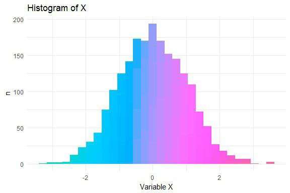
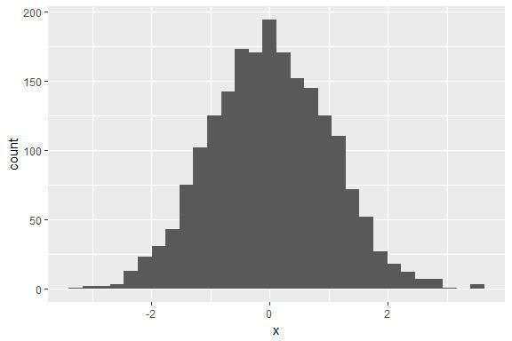
In this post you’ll learn how to create histograms like this:

The data

Let’s simulate data for a continuous variable x in a data frame d:

set.seed(070510)
d <- data.frame(x = rnorm(2000))

head(d)
>            x
> 1  1.3681661
> 2 -0.0452337
> 3  0.0290572
> 4 -0.8717429
> 5  0.9565475
> 6 -0.5521690

Basic Histogram

Create the basic ggplot2 histogram via:

library(ggplot2)

ggplot(d, aes(x)) +
    geom_histogram()

Adding Colour

Time to jazz it up with colour! The method I’ll present was motivated by my answer to this StackOverflow question.

We can add colour by exploiting the way that ggplot2 stacks colour for different groups. Specifically, we fill the bars with the same variable (x) but cut into multiple categories:

ggplot(d, aes(x, fill = cut(x, 100))) +
    geom_histogram()

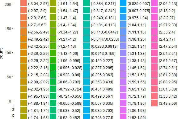
What the…

Oh, ggplot2 has added a...

@drsimonj here to introduce my latest tidy-modelling package for R, “twidlr”. twidlr wraps model and predict functions you already know and love with a consistent data.frame-based API!

All models wrapped by twidlr can be fit to data and used to make predictions as follows:

library(twidlr)

fit <- model(data, formula, ...)
predict(fit, data, ...)

• data is a data.frame (or object that can be corced to one) and is required
• formula describes the model to be fit

The motivation

The APIs of model and predict functions in R are inconsistent and messy.

Some models like linear regression want a formula and data.frame:

lm(hp ~ ., mtcars)

Models like gradient-boosted decision trees want vectors and matrices:

library(xgboost)

y <- mtcars$hp
x <- as.matrix(mtcars[names(mtcars) != "hp"])

xgboost(x, y, nrounds = 5)

Models like generalized linear models want you to work. For...

@drsimonj here to show you how to conduct ridge regression (linear regression with L2 regularization) in R using the glmnet package, and use simulations to demonstrate its relative advantages over ordinary least squares regression.

Ridge regression

Ridge regression uses L2 regularisation to weight/penalise residuals when the parameters of a regression model are being learned. In the context of linear regression, it can be compared to Ordinary Least Square (OLS). OLS defines the function by which parameter estimates (intercepts and slopes) are calculated. It involves minimising the sum of squared residuals. L2 regularisation is a small addition to the OLS function that weights residuals in a particular way to make the parameters more stable. The outcome is typically a model that fits the training data less well than OLS but generalises better because it is less sensitive to extreme...

@drsimonj here to show you how to do leave-one-out cross validation using pipelearner.

Leave-one-out cross validation

Leave-one-out is a type of cross validation whereby the following is done for each observation in the data:

• Run model on all other observations
• Use model to predict value for observation

This means that a model is fitted, and a predicted is made n times where n is the number of observations in your data.

Leave-one-out in pipelearner

pipelearner is a package for streamlining machine learning pipelines, including cross validation. If you’re new to it, check out blogR for other relevant posts.

To demonstrate, let’s use regression to predict horsepower (hp) with all other variables in the mtcars data set. Set this up in pipelearner as follows:

library(pipelearner)

pl <- pipelearner(mtcars, lm, hp ~ .)

How cross validation is done is handled by learn_cvpairs()...

@drsimonj here to show you how to use ggraph and corrr to create correlation network plots like these:

ggraph and corrr

The ggraph package by Thomas Lin Pedersen, has just been published on CRAN and it’s so hot right now! What does it do?

“ggraph is an extension of ggplot2 aimed at supporting relational data structures such as networks, graphs, and trees.”

A relational metric I work with a lot is correlations. Becuase of this, I created the corrr package, which helps to explore correlations by leveraging data frames and tidyverse tools rather than matrices.

So…

• corrr creates relational data frames of correlations intended to work with tidyverse tools like ggplot2.
• ggraph extends ggplot2 to help plot relational structures.

Seems like a perfect match!

Libraries

We’ll be using the following libraries:

library(tidyverse)
library(corrr)
library(igraph)
library(ggraph)

@drsimonj here to show you how to use xgboost (extreme gradient boosting) models in pipelearner.

Why a post on xgboost and pipelearner

xgboost is one of the most powerful machine-learning libraries, so there’s a good reason to use it. pipelearner helps to create machine-learning pipelines that make it easy to do cross-fold validation, hyperparameter grid searching, and more. So bringing them together will make for an awesome combination!

The only problem - out of the box, xgboost doesn’t play nice with pipelearner. Let’s work out how to deal with this.

Setup

To follow this post you’ll need the following packages:

 Install (if necessary)
install.packages(c("xgboost", "tidyverse", "devtools"))
devtools::install_github("drsimonj/pipelearner")

 Attach
library(tidyverse)
library(xgboost)
library(pipelearner)
library(lazyeval)

Our example will be to try and predict whether tumours...

@drsimonj here to show you how to use pipelearner to easily grid-search hyperparameters for a model.

pipelearner is a package for making machine learning piplines and is currently available to install from GitHub by running the following:

 install.packages("devtools")   Run this if devtools isn't installed
devtools::install_github("drsimonj/pipelearner")
library(pipelearner)

In this post we’ll grid search hyperparameters of a decision tree (using the rpart package) predicting cars’ transmission type (automatic or manual) using the mtcars data set. Let’s load rpart along with tidyverse, which pipelearner is intended to work with:

library(tidyverse)
library(rpart)

The data

Quickly convert our outcome variable to a factor with proper labels:

d <- mtcars %>% 
  mutate(am = factor(am, labels = c("automatic", "manual")))
head(d)
>    mpg cyl disp  hp drat    wt  qsec vs        am gear

@drsimonj here to share my big takeaways from rstudio::conf 2017. My aim here is to share the broad data science opinions and challenges that I feel bring together the R community right now, and perhaps offer some guidance to anyone wanting to get into the R community.

DISCLAIMER: this is based on my experience, my primary interests, the talks I attended, the people I met, etc. I’m also very jet lagged after flying back to Australia! If I’ve missed something important to you (which I’m sure I have), please comment in whichever medium (Twitter, Facebook, etc.) and get the discussion going!

My overall experience

I’ll start by saying that I had a great time. RStudio went all out and nailed everything from getting high-quality speakers, to booking a great venue and organizing a social event at Harry Potter world I won’t forget. But if I do, Hilary Parker took some great shots!

Here are...

@drsimonj here to introduce pipelearner – a package I’m developing to make it easy to create machine learning pipelines in R – and to spread the word in the hope that some readers may be interested in contributing or testing it.

This post will demonstrate some examples of what pipeleaner can currently do. For example, the Figure below plots the results of a model fitted to 10% to 100% (in 10% increments) of training data in 50 cross-validation pairs. Fitting all of these models takes about four lines of code in pipelearner.

Head to the pipelearner Github page to learn more and contact me if you have a chance to test it yourself or are interested in contributing (my contact details are at the end of this post).

Examples

Some setup

library(pipelearner)
library(tidyverse)
library(nycflights13)

 Help functions
r_square <- function(model, data) {
  actual    <-

@drsimonj here to share a tidyverse method of grid search for optimizing a model’s hyperparameters.

Grid Search

For anyone who’s unfamiliar with the term, grid search involves running a model many times with combinations of various hyperparameters. The point is to identify which hyperparameters are likely to work best. A more technical definition from Wikipedia, grid search is:

an exhaustive searching through a manually specified subset of the hyperparameter space of a learning algorithm

What this post isn’t about

To keep the focus on grid search, this post does NOT cover…

• k-fold cross-validation. Although a practically essential addition to grid search, I’ll save the combination of these techniques for a future post. If you can’t wait, check out my last post for some inspiration.
• Complex learning models. We’ll stick to a simple decision tree.
• Getting a great model fit. I’ve...